NUANCES-FARMSIM

NUANCES-FARMSIM (FArm-scale Resource Management SIMulator) is an integrated crop – livestock model developed to analyse African smallholder farm systems.

The model modules

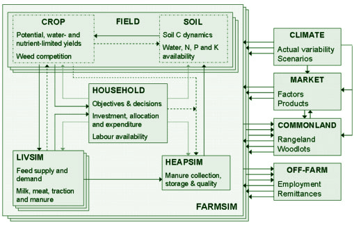
A schematic representation of the relationships between different modules of the model FARMSIM (FArm-scale Resource Management SIMulator). Crop and soil models are combined within the FIELD module; different instances of FIELD represent the various field plots of a farm. Different instances of LIVSIM (the LIVestock SIMulator) represent different herds of cattle, sheep, goats or individual animals. Different instances of FARMSIM represent farm types of different resource endowment. Weather conditions, markets and common resources are driving variables to the farm system.

NUANCES-FIELD

FIELD uses a simple approach with a seasonal time step: i) to simulate water and macronutrient dynamics in the soil and supply to crops, ii) to calculate crop yields from calculated water and nutrient availabilities, and iii) to monitor indicators of resource degradation, such as soil organic matter dynamics and soil erosion. The FIELD module readily can be parameterised for a variety of crops (to date we have included maize, grain legumes, sweet potato, cotton, and Napier grass) and a variety of soil types. Different combinations of crops and soils can be simulated to explore the interactions occurring within the farm for different field types (e.g. infields and outfields, annual and perennial crops, etc.). The most important state variables that are followed in time are linked to soil fertility: organic carbon, total nitrogen, available phosphorus and exchangeable potassium stocks. Per season crop yield is calculated using current soil fertility and external inputs like manure and mineral fertiliser. More than one field in the farm can be simulated: the user can determine the number of fields and their size, the soil characteristics and the crop that is grown on each field. For fodder crops (e.g. Napier grass), FIELD was adapted to run on two-monthly time steps in order to simulate regular cuttings. By dividing the field of Napier grass in different sections, ranges of cutting intervals can be simulated and every month Napier grass can be fed to the animals if needed, according to the characteristics of the crop-livestock system. Recently the model has been adapted to incorporate QUEFTS

NUANCES-LIVSIM

LIVSIM is an individual based livestock production model that simulates animal production (meat, milk, progeny and manure) and maintenance requirements. Different livestock units can be taken into account, each characterised by production objectives (dairy, meat, manure, traction), animal species and breeds. The model runs on a monthly basis, and can be used in either a deterministic or a stochastic version. The state variables of the module are the age, weight and reproductive status of the animal. Per month the production by the animals is calculated. 

NUANCES-HEAPSIM

The dynamics of nutrients via manure collection, storage and use as well as changes in quality due to management are simulated by the module HEAPSIM, which considers the transfer efficiencies for the different processes under different livestock production systems, types of storage and handling facilities. This module also runs on a monthly basis. 

NUANCES-LABOURSIM

Labour is an important limiting resource in many smallholder farming systems. In the model labour is not treated as a dynamic variable but as a resource that is internally available (as a consequence of members of the family working on the farm) and as an external resource that can be hired in. The model keeps track of a monthly balance of labour availability, to capture the variability of demand and availability of this resource within the year. 

The total amount of labour available per month (expressed in man-days, and resulting from the sum of internally available and externally hired labour) is allocated to different activities. The labour allocated to an activity affects the outcomes simulated by the models of the different subsystems (i.e. livestock, crop and soil and manure management). For each of the modules a set of key activities is defined, and the amount of labour that is needed for performing each of these activities is quantified. As several of these activities take place at certain moments in the year, for example weeding the maize fields only takes place in the second and third month after planting the maize, this leads to a temporal variability in the demand for labour needed to perform the activities as best practices (i.e. without loss of productivity). These monthly values for the demand of labour are compared with the monthly values of labour availability. If in each month labour availability is larger or equal to labour demand, no reduction takes place in the biophysically-determined values of production (e.g. crop production, livestock production and manure production in HEAPSIM). If in certain months not enough labour is available to cover labour demand for best practices, a decision is made on how the limited resource labour is allocated, and which activities are given priority. 

For those activities for which demand is not covered by the amount of labour allocated to them, the biophysically determined levels of production are reduced by multiplying them by a ‘labour reduction factor’. This reduction factor is a function of the amount of labour allocated to the activity and depends further on the type of activity. For example, in LIVSIM the reduction factor affects the amount of feed that can be collected for the cattle. In FIELD insufficient labour affects different activities depending on the timing of the labour constraint, as the consequences of not investing enough labour in either planting and ploughing, weeding, harvesting or erosion control measures are different. The timing of these activities within FIELD is not fixed, but depends on which crops are grown.  The model is set up in such a way that if a certain crop is chosen, certain activities automatically need to take place within specific periods during the season. Depending on the size of the field a certain amount of labour is required to achieve the biophysically-determined attainable crop yield. A lack of labour for a certain activity at a certain moment leads to a reduced crop yield (in the case of planting, weeding and harvesting), or to increased soil erosion (if the labour necessary for erosion control measures is insufficient). 

The way this yield reduction is calculated is simple. For, for example, weeding, the relationship between labour and yield reduction is defined by the amount of labour (expressed as man-days per month per ha allocated to that activity) needed to perform the activity as best practice (i.e. no yield reduction) and the yield reduction that occurs when no labour is invested into that activity. For a given labour availability in between these labour settings, the yield reduction is calculated proportionally to the difference between the labour availability and the labour availability needed for best practice using the yield reduction with no labour input. With more labour available than the labour needed for best practice the yield reduction is of course zero. This simple approach has been tested in maize weeding experiments in Bukoba, Tanzania, and showed to be a good approach to model the interaction between labour and yield reduction. The amount of labour available for planting and ploughing per ha of land is linked to the delay of crop planting as compared with the optimal start of the growing season. This delay is an input variable for the FIELD module, which uses it to adjust the availability of nutrients in the soil for the crop and the potential light interception. The relationships between planting date and the availability of nutrients and light interception are based on simulations with detailed process-based models like LINTUL and APSIM.

This setup of the labour module allows the user to simulate the effects of labour on the productivity of the subsystems in a semi-dynamic way (i.e. considering the timing of activities during the season) without substantial increases in model complexity and data demands. For example, FIELD operates on a seasonal time-step, but thanks to the linkage of the cropping calendar to the timing of certain activities, the overall effects of labour shortages at specific moments in the year or season can be taken into account. Further, it is possible to identify the critical moments in the year in which labour availability is a major constraint. Therefore we can use the simple summary model FIELD which has a small data demand and which is easily parameterised for different crop growing conditions, whilst capturing the key effects of variability in labour availability. 

Interactions between modules

Exchange between the modules takes place at different moments during the year. Manure produced in the manure heap is applied at the beginning of each rainy season to the different fields, depending on the decisions taken by the farmer. Based on this information, the state of the soils of the different fields, the input in terms of mineral fertiliser and labour and the meteorological driving variables, the crop and fodder production of that rainy season is calculated. Using this information then LIVSIM and HEAPSIM are run. This gives the availability of manure for the next season, with which the production of the different fields can be calculated, which is the input for LIVSIM and HEAPSIM, etc. All the flows of resources between the modules are determined by decision-rules. These decision rules are determined by the description of the smallholder system under study and by the type of analysis proposed. For example, a rule could be that all above-ground crop residues are taken from the field, fed to a zero-grazing cow and the refusals of the cow added to the manure heap. This automatically determines how the modules interact and how much of each resource flows from module to module. Maize thinnings fed to the animals are monitored, and we took the simple approach of reducing the yield of maize at the end of the season by the amount fed to the animals, thereby assuming no improved production of the maize that was left as a consequence of the reduced density. No other resources flow between these two compartments within the cropping season.

    One of the most important flows between modules is the flow of organic matter. Starting from LIVSIM, manure is produced and refusals are calculated based on the difference between actual feed intake of the animals and the amount of fodder on offer. These monthly values of fresh manure and refusals collected with a certain efficiency are inputs to the module HEAPSIM. HEAPSIM calculates the losses of carbon, nitrogen, phosphorus and potassium due to decomposition, gaseous losses and leaching. After six months the composted manure and refusals in the heap are applied to the fields, following different possible allocation rules. The manure can, for example, be spread evenly over all the fields, or concentrated on the best fields. Based on climate, on the existing soil nutrient availability, and the availability of nutrients from the applied manure applied and/or mineral fertilisers, the FIELD module calculates crop yield and changes in the soil state variables. This yield is reduced if labour is insufficient for all best practices. Based on the actual yield of both fodder and food crops, crop residue biomass is calculated and decisions are made (see below) with regard to the fraction of this that remains in the field, is stored, or is fed directly to the animals.            

Setup of the decision making module

The core of FARMSIM is formed by the different modules described in the previous section. In FARMSIM the decision module is outside of this core, and serves to supply the necessary input to make the modules run and communicate with each other. The decision module supplies the necessary input parameters that determine how resources should be allocated on a monthly or seasonal basis over the different components of the farm and the different activities that should take place. The core of FARMSIM in which all the modules are linked then calculates the consequences of these decisions for that specific growing season, using also all the other inputs necessary for running the model. The results of this model run are then reported back to the decision module. 

Depending on the specific interests of the user, different types of analyses can be performed with the decision module:

• A fixed scenario analysis can be performed, in which the consequences of a fixed strategy are calculated over a certain time span. The same decision parameters as specified in the decision module are used every season throughout the simulated period, and the farm is followed in time to evaluate the impacts of such strategy.  
• State-based decision making, in which decisions change (and decision parameters are adapted) depending on the state variable that is simulated (e.g. soil fertility or cash availability). The implementation of such decision can be done using, for example, a simple rule – based approach, or by building in a more complex Linear Programming decision tool.
• Optimization of decisions and strategies using inverse modelling techniques, in which the model outputs for a chosen strategy are evaluated, and on the basis of these outputs these strategies can be optimized, or ‘acceptable’ farming strategies be identified.     

 

Additional information, as well as the latest version of FarmSim can be downloaded from : http://models.pps.wur.nl

FarmSim Models & Data